How to extract data from the Fabric Metrics App – Part 1

In recent discussions with my customers about Microsoft Fabric, the questions pops up how to create an internal and fair charge-back mechanism. There are different possibilities, from user-based, item-based, or usage-based scenarios, which you can leverage. From my point of view, the usage-based model would be the fairest one. In such a scenario, creators of items are eager to optimize their workload to reduce the usage on a capacity and therefore save some cost. But how can you create such a charge-back report? Let me walk you through in a this blog post how to set the basics and in my next one how a possible solution can look like.

Prerequisites

To be able to collect the necessary data and create a charge-back report, we will need some tools and items.

Let’s get started

The Fabric Capacity Metrics App is the best way to get an overview of who created how much load with which items on your capacity. The Microsoft documentation shows how easy it is to install and use it. Once installed, I switch to the Workspace called Microsoft Fabric Capacity Metrics and change the workspace settings to assign a capacity to the workspace. In my case, I use a Fabric one but a Premium, Premium per User, or Embedded would work as well.

Once done, I refresh the Semantic Model and open the report afterwards. Now, I have already an overview of the usage of the last 14 days. I would be able to filter now for example on a specific day to see what kind of items have produced how much load. But as I wish to have in detail who created the load, I need to drill-down to a specific data point. For that, I select on the top right visual a data point and hit the Explore button.

On the next page, I have a good overview of all interactive and background operations that have happened on my capacity (the two table visuals in the middle). If you’re interested in what kind of operations are considered as interactive resp. background, feel free to check the Microsoft documentation.

The issue right now is that on one hand we have only the last 14 days data and usually a monthly charge-back report is needed. An on the other hand, the details are only per Timepoint, which is a 30 second interval, available. Therefore, I need to extract the data to have a longer history and do that for each timepoint of the day. Let me start with extracting the data first.

Capture the DAX statement

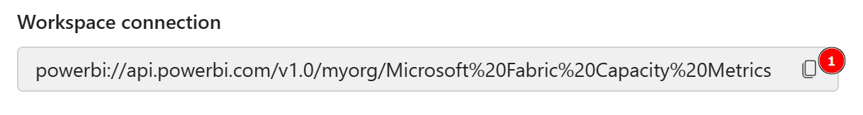
I could connect with DAX Studio to the Semantic Model as the workspace is sitting now in a capacity and try to write my own DAX statement to get the required details. But as I’m efficient (not lazy as Patrick LeBlanc from Guy in a Cube says ;)), I’ll capture rather the DAX statement and adjust it if needed. To do so, I’ll use the SQL Profiler and connect to the Semantic Model. To get the connection string, I switch back to the Workspace settings, select Premium, and scroll down until I see the connection string. By hitting the button to the right, I copy it.

Now, I open SQL Server Profiler and put the connection string as Server name, select Azure Active Directory – Universal with MFA as authentication method, put in my mail as User name and hit Options.

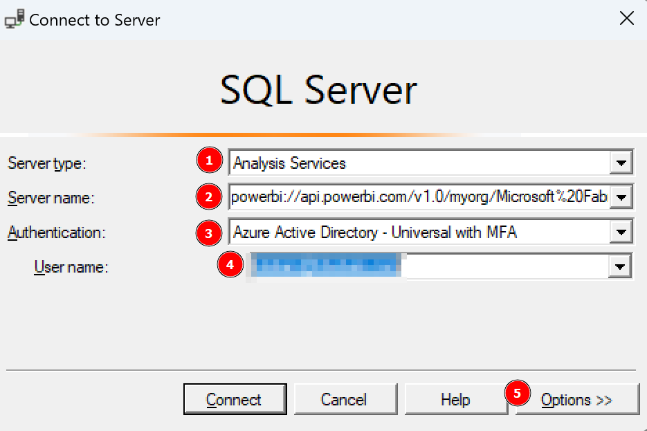
Once the window extends, I select Connection Properties, specify Fabric Capacity Metrics as database to which I wish to connect, and hit Connect.

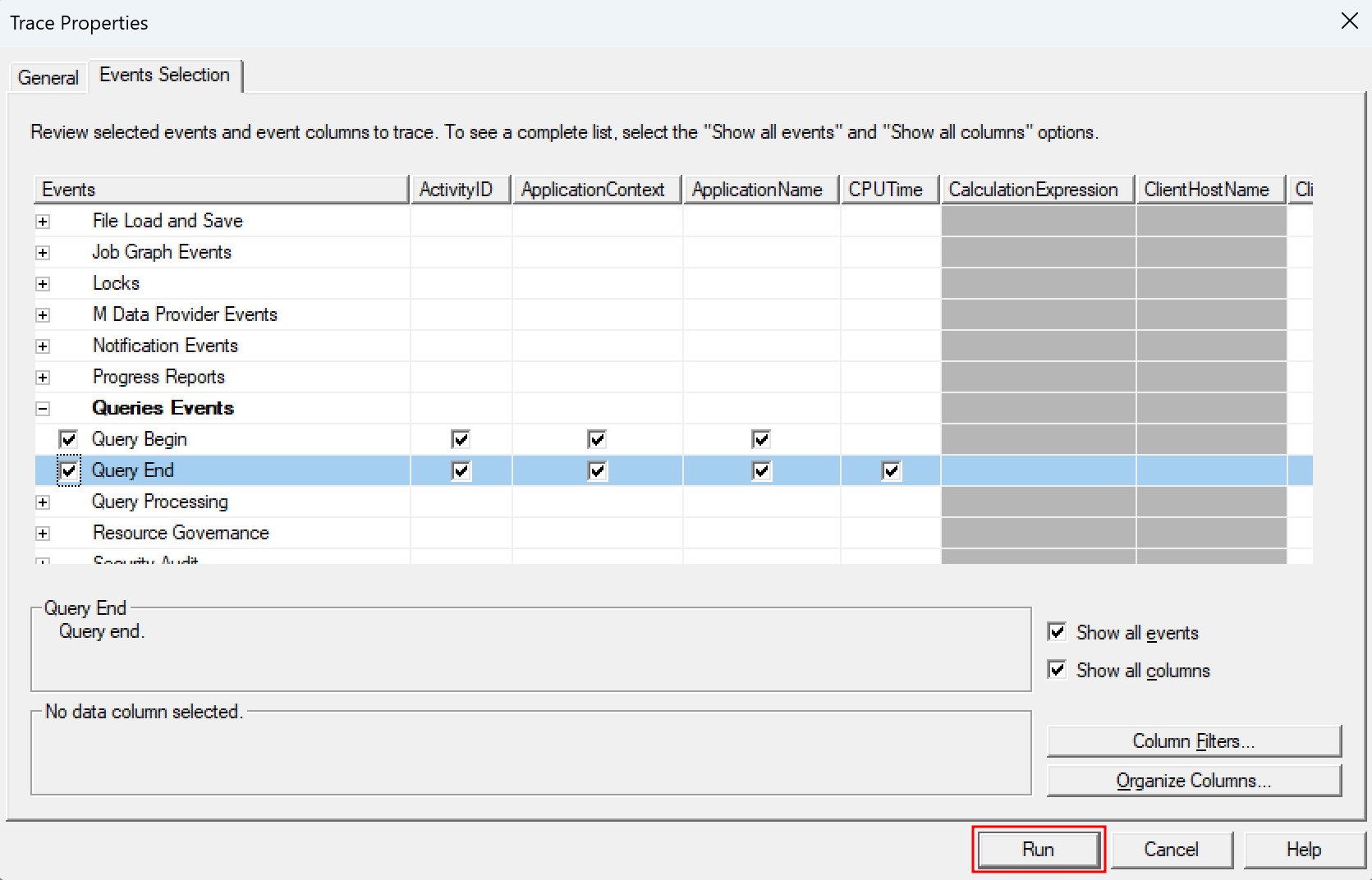
On the next screen, I go directly to Events Selection at the top, extend Queries Events, and select Query Begin and Query End.

With that, I’m prepared to capture the DAX query but I don’t hit Run yet. I wish to make sure to get the right query so I switch back to the Power BI Report and enter the edit mode. Now, I just delete all the visuals except the Interactive Operations table. This way, I make sure no other query is executed and I capture only what I need.

Once prepare, I switch back to SQL Profiler and hit Run.

After our tracer is running, I switch one more time back to the Power BI Report and hit the refresh button at the top right.

Now I see two operations in my Tracer – Query Begin and Query End. If I select one of it, I have now the DAX Query for the interactive Operations.

DEFINE
	MPARAMETER 'CapacityID' = 
		"9C3E7404-D2DA-4CB6-B93F-9873BDD3D95A"

	MPARAMETER 'TimePoint' = 
		(DATE(2024, 3, 20) + TIME(15, 59, 0))

	VAR __DS0FilterTable = 
		TREATAS({"9C3E7404-D2DA-4CB6-B93F-9873BDD3D95A"}, 'Capacities'[capacityId])

	VAR __DS0FilterTable2 = 
		TREATAS({"Dataset"}, 'Items'[ItemKind])

	VAR __DS0FilterTable3 = 
		TREATAS(
			{(DATE(2024, 3, 20) + TIME(15, 59, 0))},
			'TimePoints'[TimePoint]
		)

	VAR __DS0Core = 
		SUMMARIZECOLUMNS(
			ROLLUPADDISSUBTOTAL(
				ROLLUPGROUP(
					'TimePointInteractiveDetail'[OperationStartTime],
					'TimePointInteractiveDetail'[OperationEndTime],
					'TimePointInteractiveDetail'[Status],
					'TimePointInteractiveDetail'[Operation],
					'TimePointInteractiveDetail'[User],
					'TimePointInteractiveDetail'[OperationId],
					'TimePointInteractiveDetail'[Billing type],
					'TimePointInteractiveDetail'[Start],
					'TimePointInteractiveDetail'[End],
					'Items'[IsVirtualArtifactName],
					'Items'[IsVirtualWorkspaceName],
					'Items'[WorkspaceName],
					'Items'[ItemKind],
					'Items'[ItemName]
				), "IsGrandTotalRowTotal"
			),
			__DS0FilterTable,
			__DS0FilterTable2,
			__DS0FilterTable3,
			"SumTimepoint_CU__s_", CALCULATE(SUM('TimePointInteractiveDetail'[Timepoint CU (s)])),
			"SumThrottling__s_", CALCULATE(SUM('TimePointInteractiveDetail'[Throttling (s)])),
			"SumDuration__s_", CALCULATE(SUM('TimePointInteractiveDetail'[Duration (s)])),
			"SumTotal_CU__s_", CALCULATE(SUM('TimePointInteractiveDetail'[Total CU (s)])),
			"Sumv__of_Base_Capacity", CALCULATE(SUM('TimePointInteractiveDetail'[% of Base Capacity]))
		)

	VAR __DS0PrimaryWindowed = 
		TOPN(
			502,
			__DS0Core,
			[IsGrandTotalRowTotal],
			0,
			[SumTimepoint_CU__s_],
			0,
			'TimePointInteractiveDetail'[Billing type],
			0,
			'TimePointInteractiveDetail'[OperationStartTime],
			1,
			'TimePointInteractiveDetail'[OperationEndTime],
			1,
			'TimePointInteractiveDetail'[Status],
			1,
			'TimePointInteractiveDetail'[Operation],
			1,
			'TimePointInteractiveDetail'[User],
			1,
			'TimePointInteractiveDetail'[OperationId],
			1,
			'TimePointInteractiveDetail'[Start],
			1,
			'TimePointInteractiveDetail'[End],
			1,
			'Items'[IsVirtualArtifactName],
			1,
			'Items'[IsVirtualWorkspaceName],
			1,
			'Items'[WorkspaceName],
			1,
			'Items'[ItemKind],
			1,
			'Items'[ItemName],
			1
		)

EVALUATE
	__DS0PrimaryWindowed

ORDER BY
	[IsGrandTotalRowTotal] DESC,
	[SumTimepoint_CU__s_] DESC,
	'TimePointInteractiveDetail'[Billing type] DESC,
	'TimePointInteractiveDetail'[OperationStartTime],
	'TimePointInteractiveDetail'[OperationEndTime],
	'TimePointInteractiveDetail'[Status],
	'TimePointInteractiveDetail'[Operation],
	'TimePointInteractiveDetail'[User],
	'TimePointInteractiveDetail'[OperationId],
	'TimePointInteractiveDetail'[Start],
	'TimePointInteractiveDetail'[End],
	'Items'[IsVirtualArtifactName],
	'Items'[IsVirtualWorkspaceName],
	'Items'[WorkspaceName],
	'Items'[ItemKind],
	'Items'[ItemName]

I could use this query already and execute it in DAX Studio – just to make sure it works as expected.

Make sure to remove the [WaitTime: 0 ms] at the end of the query if you’re copying it from SQL Profiler.

Looks good! I repeat the same steps for the background operations and test is as well in DAX Studio. Once done, I close SQL Server Profiler as tracing is not necessary anymore.

As a next step, let me analyze the generated query and optimize it. I will start this time with the background operations. The first variable defined is a MPARAMETER for the Capacity ID. The second one is as well a MPARAMETER for the Timepoint including the conversion. MPARAMETERS are so-called binding parameters which are passed through from the Power BI report to Power Query. DAX.guide has a great explanation and example here: https://dax.guide/st/mparameter/ This means we have to pass those two values to retrieve the correct result.

Going further, three different variables are defined which are used later on to filter. We have again the Capacity ID, Timepoint, and an Item filter to get only Datasets. As I don’t need the Item filter, I just delete it. For readability reasons, I also renamed the other two variables going from __DS0FilterTable to varFilter_Capacity and from DS0FilterTable3 to varFilter_TimePoint.

My first block of DAX looks like this.

DEFINE
	MPARAMETER 'CapacityID' = 
		"9C3E7404-D2DA-4CB6-B93F-9873BDD3D95A" --add your capacity ID here

	MPARAMETER 'TimePoint' = 
		(DATE(2024, 3, 20) + TIME(15, 59, 0))

	VAR varFilter_Capacity = 
		TREATAS({"9C3E7404-D2DA-4CB6-B93F-9873BDD3D95A"}, 'Capacities'[capacityId]) --add your capacity ID here

	VAR varFilter_TimePoint = 
		TREATAS(
			{(DATE(2024, 3, 20) + TIME(15, 59, 0))},
			'TimePoints'[TimePoint]
		)

Replace the three dots with your Capacity ID.

The next big block is a simple group by logic based on different columns and summarizes different KPIs on top. I simplify and store it as well into a variable.

VAR varTable_Details =
		SUMMARIZECOLUMNS(
			'TimePointBackgroundDetail'[OperationStartTime],
			'TimePointBackgroundDetail'[OperationEndTime],
			'TimePointBackgroundDetail'[Status],
			'TimePointBackgroundDetail'[Operation],
			'TimePointBackgroundDetail'[User],
			'TimePointBackgroundDetail'[OperationId],
			'TimePointBackgroundDetail'[Billing type],
			'Items'[WorkspaceName],
			'Items'[ItemKind],
			'Items'[ItemName],
			
			varFilter_Capacity,
			varFilter_TimePoint,
			
			"Timepoint CU (s)", SUM('TimePointBackgroundDetail'[Timepoint CU (s)]),
			"Duration (s)", SUM('TimePointBackgroundDetail'[Duration (s)]),
			"Total CU (s)", CALCULATE(SUM('TimePointBackgroundDetail'[Total CU (s)])),
			"Throttling", CALCULATE(SUM('TimePointBackgroundDetail'[Throttling (s)])),
			"% of Base Capacity", CALCULATE(SUM('TimePointBackgroundDetail'[% of Base Capacity]))
		)

Lastly, we need an EVALUATE to get a result.

EVALUATE  SELECTCOLUMNS(
    varTable_Details,
    "BillingType", [Billing type],
    "Status", [Status],
    "OperationStartTime", [OperationStartTime],
    "OperationEndTime", [OperationEndTime],
    "User", [User],
    "Operation", [Operation],
    "OperationID", [OperationId],
    "WorkspaceName", [WorkspaceName],
    "Item", [ItemKind],
    "ItemName", [ItemName],
    "TimepointCUs", [Timepoint CU (s)],
    "DurationInS", [Duration (s)],
    "TotalCUInS", [Total CU (s)],
    "Throttling", [Throttling],
    "PercentageOfBaseCapacity", [% of Base Capacity]	
)

This way, we have now an optimized and more readable DAX statement for the Background operations. To get the same optimized query for interactive operations, I only need to replace the TimePointBackgroundDetail table with TimePointInteractiveDetail and I’m already good to go! The whole DAX statement can be found in my GitHub repo.

Now, we have everything on hand to extract the required details on a – for example – daily base. There are various options to achieve it – from Power Automate Flows, to Microsoft Fabric Pipelines, and / or Python Notebooks (Databricks or Microsoft Fabric), and many more. In my next blog post, I’ll walk you through one possible option to store the data into OneLake.

Please let me know if this post was helpful and give me some feedback. Also feel free to contact me if you have any questions.

If you’re interested in the files used in this blog check out my GitHub repo https://github.com/PBI-Guy/blog

Create a custom partition in Power BI and trigger a refresh with Python

Working with large datasets I almost always get the question if an incremental refresh can be configured within Power BI and yes, this is possible as described here. Especially if you have a date or datetime column it makes sense to set up an incremental refresh to reduce your dataset refresh time. Once set up, Power BI will create automatically some partitions behind the scenes making sure the data is stored as configured. For example if you wish to have 5 years of archived data, each year will represent one partition. But what if you don’t have a date/datetime column or you wish to create your own partition? Can you still create your own, custom partitions and trigger some kind of incremental refresh? Yes you can! Let me show you how.

Let’s quickly demystify the term “partition”

Asking chatGPT what a partition in Power BI is, we got following reply:

In Power BI, a partition is a way to break up a large dataset into smaller, more manageable chunks based on a set of defined criteria. This can be particularly useful when working with datasets that contain millions or billions of rows, as it can help to optimize performance and reduce the time it takes to load and process the data.

Partitions are essentially subsets of the data that are stored separately from the main dataset, based on specific conditions such as date ranges or other data attributes.

By dividing a large dataset into smaller partitions, Power BI can improve query and report performance, and also reduce the resources required to process and manage the data. This can lead to faster report rendering times, reduced memory usage, and improved overall user experience.

Overall, using partitions in Power BI can be a powerful way to optimize large datasets and improve the performance of your reports and visualizations.

chatGPT on “Explain what partitions are for Power BI datasets”

I must admit I don’t have anything to add here.

Let’s get started

For my demo purpose I’m going to create a dummy table in Azure SQL on which I can test custom partitions in Power BI. Further, I’ll need the open-source tool Tabular Editor (regardless if version 2 or 3) in which I’ll create my partitions. If you prefer, you can also use SQL Server Management Studio (SSMS) to create your partitions. Lastly, I’m going to use Synapse Notebooks to run my Python script at the end to trigger a partition refresh.

So let’s start and create a dummy table. I created a SQL script which will create a table with an ID, Country, Region, and a random Revenue. To update which country should be involved, you can add, delete, or modify the countries starting from line 28. If you wish to modify the schema and table name, just update it on line 36 & 37. Lastly, I specify how many rows per country should be added. In my case I add 10 rows per country but if you need more (or less) update the CounterMax variable on line 39.

Once executed, I got 70 rows in my case in my newly created SQL table. Now, let’s connect with Power BI Desktop to it and switch to Power Query (Transform Data button once connected to the SQL table). Why Power Query? Because I’ll prepare my first partition there and will reuse the code for my other partitions.

As you can see in the screen shot above I don’t have a filter applied yet and see the full list of all my countries. To make my solution as configurable as possible, I add a new parameter called “Europe” and one called “America”. I choose Text as type and add the Europe resp. America as Current Value.

The parameters screen shot shows two further parameters called “SQL Server Name” and “Database Name”. I parametrized my data source for reusability and is considered as best practice but it’s not mandatory.

Next, I select my table, choose the little arrow in the right corner of the column, select Text Filters – Equals… and choose my Europe parameter. Once done, I confirm by selecting OK.

Now, I select Advanced Editor in the ribbon and copy the whole code behind. Making sure I’ll not lose the code I paste it into Notepad.

Lastly, I close the Advanced Editor and confirm everything by hitting “Close & Apply” to load the data into Power BI. After data has loaded, I publish my Power BI report to a Premium workspace (PPU or Embedded works as well).

Once published, I switch to Power BI Service, select the workspace in which the report has been published, head over to settings, and copy the workspace connection.

Next, I open External Tools, connect to my workspace, and select the custom partition dataset. In there, you will find one partition if you expand Tables – Your Table Name (Custom Partition in my case) – Partitions. If you select it, you’ll find the M-Code in the Expression Editor on the right hand side.

Let’s now build our own partition with the same approach but in Tabular Editor. All I need to do is right-click on Partitions, select New Partition (Power Query), click afterwards my newly created partition, and paste the M-Code into the Expression Editor. Lastly, I just need to update the “Europe” parameter to “America”. Make sure the name matches exactly with your parameter name. If you wish to double check it, just expand “Shared Expressions” which represents your defined parameters in Power BI.

To make the partitions more user-friendly, let’s rename them as well by just selecting it and hit F2. I renamed it to “Europe” and “America”. Once done, save your data model.

If I check my report now, nothing has changed as I haven’t refreshed my dataset yet. So let’s trigger a manual refresh in Power BI Service and check the report if something has changed. As we can see, all countries from the region America are now also included. Nice!

Let’s now try to trigger a partition refresh instead of the whole table. In one of my previous blog posts I showed how to refresh a Dataset with Python. I’m going to use the same code and just adjust it a little bit. Checking the documentation we can add a body to our POST request and define which partition should be refreshed. Therefore I adjust my Python script by adding following parameter before calling the REST API.

body = {
    "type": "full",
    "commitMode": "transactional",
    "maxParallelism": 3,
    "retryCount": 1,
    "objects": [
        {
            "table": "Custom Partition",
            "partition": "Europe"
        }
    ]
}

After I executed the script and check the Refresh history of the dataset in Power BI Service, I’ll see Via Enhanced Api as Type.

But how do I know that only one partition is now refreshed and not the whole table? I can check that either with Tabular Editor or SSMS. In Tabular Editor I just connect again to my Dataset, select my Europe partition and check the “Last Processed” Date and Time. If I compare the Date and Time with my America partition I see a difference – so it worked!

With SSMS I have also to connect to my Dataset, right click on my Table, select Partitions, and then I will be able to see the different Partitions as well as the Last Processed Date and Time. By the way you could also manually trigger a Partition Refresh from this view by just selecting the process button (it’s the small one with the three green arrows) and confirm on the next screen with OK.

As a final step let’s test a little bit the performance as well as what would happen if we add a new region. Let’s first add the Asia region with some countries. To do so I open my SQL statement again and add China, Japan, and India as Asia countries.

Once successfully executed, I have 100 rows in my Custom Partition table as each new country added 10 rows. Let’s refresh the Power BI Dataset and check if I’ll see the newly added countries in my report. And as expected, nothing has changed in my report meaning the Asia region is not included! This makes sense as the two created partitions only include America and Europe, therefore everything else will be filtered out. This means I need to create another partition either for each Region or I create “everything else” partition. In my case and for the demo purpose, I choose the second option. To do so I open my report in Desktop, switch to Power Query, click the gear icon in my Filtered Rows step under Applied Steps, and configure the filter to does not equal to Europe And does not equal to America parameter.

Once applied with OK I’ll see a Preview of my Asia countries coming from SQL. Following the steps described above, I just copy the whole M-Code from the Advanced Editor window, switch to Tabular Editor (or SSMS), and create a new Partition with this code called “All other Regions”. After saving my data model I switch back to Power BI Service and trigger a full refresh manually. And now my three new countries are also included in my report.

As we have now three different partitions and making sure we’ll get all data which are added to the SQL table, let’s do some performance testing. I’ll always follow the same approach:

  1. Add the same number of rows to each partition (I deleted France from my SQL table making sure each region has 3 countries)
  2. Do a single partition refresh and check how long it takes
  3. Refresh all partitions at the same time and check how long it takes
  4. Do a full refresh and check how long it takes

As I’m interested if there is a difference refreshing the whole data model or explicitly calling the REST API and trigger all partitions at once, I decided to differentiate step 3 and 4.

You can also trigger multiple partition refreshes through the API by adjusting the body. In my case I used the below body.

body = {
    "type": "full",
    "commitMode": "transactional",
    "maxParallelism": 3,
    "retryCount": 1,
    "objects": [
        {
            "table": "Custom Partition",
            "partition": "Europe"
        },
        {
            "table": "Custom Partition",
            "partition": "America"
        },
        {
            "table": "Custom Partition",
            "partition": "All other Regions"
        }
    ]
}

To add new rows I’ll use my SQL script and adjust the CounterMax Parameter to different values.

Keep in mind, the bigger the number is, the longer it will run. After having roughly 1 Mio rows I used the INSERT INTO SQL Statement to just duplicate the data instead of running the script as it would take too long to add so many rows.

And here is my result. As you can see trigger a single partition is always faster then refreshing the whole dataset. Well, this is expected. But the time saved varies between 37 – 72%! The bigger the data, the more time you’ll save. Interestingly enough, triggering all partitions via the REST API to refresh is also faster, but the bigger the data gets the less time you’ll save with it but still worth considering from my point of view.

Please let me know if this post was helpful and give me some feedback. Also feel free to contact me if you have any questions.

If you’re interested in the files used in this blog check out my GitHub repo https://github.com/PBI-Guy/blog